Let the Vector Index Drive: ScaNN on AlloyDB

The Google Cloud write-up about Lucius mentions one query that went from 1.14 seconds to 24 milliseconds on AlloyDB. This is the long version of that one query: what the slow shape looked like, why the ScaNN index sat unused, what the rewrite changed, how each number was measured, and two things that went wrong after the rewrite and are still open. Every figure below comes from the production database on 22 September 2026 or from the code and the commits that shipped the changes, and the section on what broke includes a number I would rather not have found.

The problem

Lucius matches public tenders to companies that could bid for them. As of 22 September 2026 the catalog holds 232,620 notices from 15 distinct sources across 179 countries, and 41,622 of them are still open by deadline. Each notice has a 3,072-dimension embedding in a tender_embeddings table in the same AlloyDB cluster: 232,714 vectors, all from the same embedding model. The matching feed and the in-app agent both call one function, search_similar_tenders, whenever they need notices like a given text.

Two facts about that table shape everything that follows. First, a 3,072-dimension float vector is 12 KB, so PostgreSQL stores it out of line: the table is 7,335 MB, of which 6,940 MB is TOAST and 132 MB is the main heap. Reading one vector to compute one exact distance costs about 23 buffer reads. Second, most vectors belong to notices nobody can bid on any more. Only 50,336 catalog rows have an active status; 177,617 are expired and 4,366 archived, and they all keep their embeddings. 182,228 of the 232,489 catalog vectors, 78 percent, sit on rows the search has to throw away.

The query before

The first version was the obvious query. Join embeddings to tenders, keep rows above a similarity threshold, restrict to the public catalog and to active status, order by cosine distance, take the top few. This is the text removed in commit 72d6028b:

SELECT t.*, 1 - (te.embedding <=> $1::vector) AS similarity
FROM tender_embeddings te
JOIN tenders t ON t.id = te.tender_id
WHERE 1 - (te.embedding <=> $1::vector) >= $2
  AND t.owner_id IS NULL
  AND (t.owner_id IS NOT NULL OR COALESCE(t.status, 'active') = 'active')
ORDER BY te.embedding <=> $1::vector
LIMIT $3;

It returned correct rows. On 31 July, an EXPLAIN ANALYZE against production with a real stored vector measured it at 1,140 ms and about 500,000 buffers per call. The plan did not touch the ScaNN index. The planner scanned tenders in parallel, looked up each row's vector by primary key to compute the distance, and sorted the lot. With a join and three filters sitting between the ORDER BY and the index, that was the path it chose.

The query after

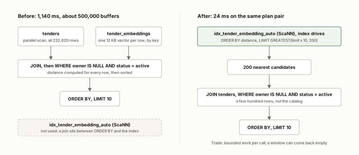
The rewrite gives the index a question it can answer on its own, then does everything else on the result. This is the shape in app/db/postgres.py today:

SELECT t.*, 1 - cand.dist AS similarity
FROM (
    SELECT te.tender_id, te.embedding <=> $1::vector AS dist
    FROM tender_embeddings te
    ORDER BY te.embedding <=> $1::vector
    LIMIT GREATEST($3 * 10, 200)
) cand
JOIN tenders t ON t.id = cand.tender_id
WHERE 1 - cand.dist >= $2
  AND t.owner_id IS NULL
  AND (t.owner_id IS NOT NULL OR COALESCE(t.status, 'active') = 'active')
ORDER BY cand.dist
LIMIT $3;

The inner query touches only the embeddings table, so the index drives it and the limit is pushed into the index scan. It asks for ten times the caller's limit, with a floor of 200, because the outer filters will drop most candidates. The join and the filters then run over a few hundred rows instead of the catalog. The callers did not change. The retrieval service passes a threshold of 0.3, and the feed asks for 80 rows:

rows = await pg.search_similar_tenders(
    embedding=vec, limit=n_results, threshold=0.3,
    owner_id=owner_id, countries=countries,
)

On 31 July the same EXPLAIN ANALYZE pair measured this shape at 24 ms. Those are the two numbers in the write-up, and the index that made them possible already existed before either was taken. The index was not the change. The query shape was.

The index

The live index is idx_tender_embedding_auto, defined as USING scann (embedding cosine) WITH (mode='AUTO'): 141 MB on disk for 232,714 vectors, on alloydb_scann 0.1.4 and PostgreSQL 18.3. Its statistics show 37,466 scans, with an average of 1,884 index tuples read and 1,762 heap tuples fetched per scan. ScaNN is the only choice at this width. pgvector's HNSW refuses columns over 2,000 dimensions, and the migration that recreates the index for the second regional cluster quotes the exact error, then builds the same index with num_leaves = 50. Inline filtering is switched on for the cluster, but the owner, status and country columns live one join away on tenders, so it cannot see the predicates that matter here.

How it was measured, and the numbers

Two methods. Plans come from EXPLAIN (ANALYZE, BUFFERS) on production, with the query vector read from a stored tender embedding rather than pasted in, run once cold and once warm, against two different anchor notices. Production means come from pg_stat_statements, whose counters were last reset on 28 August, so the window is 28 August to 22 September. One trap in that view: the cluster's own tooling records a zero-time copy of each statement under the same query id and a different role, so the means below count only the backend's own rows.

The rewritten shape, in that window: 10,204 calls, mean 172 ms, about 26,800 buffers per call, 1.1 percent of all database time. A live plan today on the first anchor: 583 ms cold, of which 506 ms was disk, then 40 ms warm over 40,366 buffers, with Limit: 200 visible inside the index scan node and 9 of the 200 candidates surviving the status filter. The index scan node accounts for 38,993 of those buffers, far more than the 200 vectors it returns would need, so the index's own search is most of the cost per call. On the second anchor: 44 ms, and 0 of 200 survived.

The old shape, run today for a like-for-like comparison, no longer produces the 31 July plan. In three runs the planner walked the ScaNN index and applied the filters on the index scan node. On the first anchor that takes 16 to 19 ms after 207 index entries, which is faster than the rewrite. On the second anchor it walks 2,077 entries before it finds ten active rows, touches 95,061 buffers and takes 952 ms, 807 ms of it disk. The old shape's cost depends on how deep the first ten active neighbours sit. The new shape's cost is fixed by the window. That is the whole trade, and it is a better one than the 31 July pair makes it look, because the losing side of the trade is real.

What broke on the way

The window can come back empty. The second anchor above is a catalog notice whose 200 nearest neighbours are all expired or archived. The rewrite answers in 44 ms with nothing; the old shape found ten matches by walking ten times deeper. The code comment calls a miss beyond the window acceptable recall for a similarity feature, and on average it is: production calls return 69 to 73 rows against the feed's limit of 80. But the average hides the shape of the failure. It is not a few rows short on every call. It is some vectors getting nothing at all.

The market-scoped branch undid the win. On 1 September I added a second branch to the same function. When a user's markets hold few active rows, an exact scan over just those rows replaces the global top-N, because a small market never reaches a global candidate window at all. The threshold was set at 20,000 rows, on the reasoning in the code comment that 20,000 distance computations take tens of milliseconds. That reasoning counted CPU and forgot the 23 buffers per vector. In the same window this branch ran 21,529 times at a mean of 922 ms, about 69,800 buffers per call, and 12.7 percent of all database time: more than ten times the cost of the shape it was meant to complement. A live plan for a 440-row market takes 23 ms warm and 243 ms cold, which is what the branch was built for. A 7,894-row market takes 470 ms warm and 2,477 ms cold over 510,782 buffers, and twelve markets hold more than 1,000 active rows, the largest 8,177. The threshold admits every one of them.

What is next

Three changes, in order of confidence. Lower the exact-scan threshold to the size the measurements support, somewhere near 1,000 rows, so the 157 markets at or under that size keep the exact path and the twelve larger ones go back to the index with the market predicate on the outer filter. For those larger markets, carry a copy of the country onto tender_embeddings so inline filtering can apply the market predicate without the join; that is an experiment, not a result. And when fewer rows survive the window than the caller asked for, widen the window once and retry, so the second anchor's empty answer becomes a slower correct one. Each will be measured the way this post was, and these numbers will be re-pulled before any of it is described as done.

The wider story of running the platform on one managed database, including the operations agent that reads it over MCP, is in the Google Cloud write-up. This post is the part that fits in a query plan.